Compare Synthetic Control methods which allows multiple outcomes

install.packages("MSCMT")
install.packages("Synth")
devtools::install_github("ebenmichael/augsynth")

library(MSCMT)
library(Synth)
library(augsynth)
library(multisynthdid)
library(tidyverse)

data("german_reunification")
german_reunification$index <- as.integer(as.factor(german_reunification$country) )
german_reunification <- as.data.frame(german_reunification)

Classical Synthetic Control

unit_ids <- unique(german_reunification$index)[-7]
dataprep_out <-
  dataprep(
    foo = german_reunification,
    predictors    = c("gdp","trade","infrate"),
    dependent     = "gdp",
    unit.variable = "index",
    time.variable = "year",
    treatment.identifier = 17,
    controls.identifier = unit_ids[unit_ids != 17],
    time.predictors.prior = 1981:1990,
    time.optimize.ssr = 1960:1989,
    unit.names.variable = "country",
    time.plot = 1960:2003
  )

synth_out <- synth(dataprep_out)

MSCMT package

df_m <- listFromLong(german_reunification, unit.variable="index", time.variable="year", unit.names.variable="country")

# define the sum of all cases

treatment.identifier <- "West Germany"
controls.identifier  <- setdiff(colnames(df_m[[1]]),
                                c(treatment.identifier))
times.dep  <- cbind("gdp"            = c(1960,1989),
                    "trade"          = c(1960,1989),
                    "infrate"        = c(1960,1989))
times.pred <- times.dep

mscmt_res <- mscmt(df_m, treatment.identifier, controls.identifier, times.dep, times.pred, seed=1)

14:25:05: Number of 'sunny' donors: 16 out of 16
14:25:05: Unrestricted outer optimum (obtained by ignoring all predictors) is 
14:25:05: FEASIBLE even when respecting the predictors.
Final rmspe: 0.03346181, mspe (loss v): 0.001119693
Optimal weights:
        USA     Austria Switzerland       Japan 
 0.26457047  0.49918982  0.17248101  0.06375869 

Augmented Synthetic Control

aug_syn <- augsynth( gdp + trade + infrate ~ W, index, year, 
                     german_reunification, progfunc = 'none', scm = T  )

Multiple outcomes and one treatment time found. Running augsynth_multiout.

summary(aug_syn)

Call:
augsynth_multiout(form = form, unit = !!enquo(unit), time = !!enquo(time), 
    t_int = t_int, data = data, progfunc = "none", scm = ..2)

Overall L2 Imbalance (Scaled):0.450  (0.296)

Average ATT Estimate:
  Outcome      Estimate lower_bound upper_bound p_val   Pre.RMSE
1     gdp -2360.7643320          NA          NA     0 310.710337
2   trade     8.0726851          NA          NA     0   7.290110
3 infrate    -0.4014653          NA          NA     0   1.930879

# Treatment
augsyn_tau = predict(aug_syn,att=T)

multi_sdid <- multi_sdid( gdp + infrate + trade ~ 1, 'W', 'country', 'year', german_reunification )

summary.multisynthdid(multi_sdid)

$estimate
[1] "multi_synthdid_obj"

$tau
                     gdp  infrate     trade
Avg. Treatment -1526.459 1.397776 0.3985817
SE              1347.822 1.488557 4.3167491

$dimensions
                                      [,1]
No. Treated units                    1.000
No. Control pool                    16.000
Effective no. controls               8.668
No. Post-treatment periods          14.000
No. Pre-treatment periods           30.000
Effective no. pre-treatment periods  1.000
No. Outcomes                         3.000

msdid_curve <- multi_synthdid_curves(multi_sdid$tau, complete = T)

Comparison of GDP

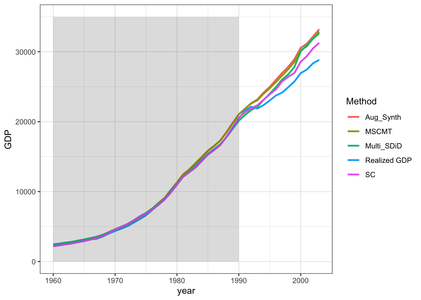
df_plot <- german_reunification %>% 
  filter( country == 'West Germany' ) %>% 
  arrange( year ) %>% 
  rename( `Realized GDP` = gdp )

df_plot <- cbind(df_plot,
                 tibble(SC = dataprep_out$Y0plot %*% synth_out$solution.w ),
                 tibble(MSCMT = as.vector( mscmt_res$data.synth$gdp) ),
                 tibble(Aug_Synth = df_plot$`Realized GDP`-augsyn_tau[,1] ),
                 tibble(Multi_SDiD = df_plot$`Realized GDP` - msdid_curve$tau_curve[1,]) )

df_plot2 <- df_plot %>% 
  select( year, `Realized GDP`, SC, MSCMT, Aug_Synth, Multi_SDiD ) %>%  #
  pivot_longer(!year, names_to = 'Method', values_to = 'GDP' )

ggplot( df_plot2, aes( x = year, color = Method, y = GDP )) + 
  geom_line( linewidth = 1 ) +
  annotate("rect", xmin = 1960, xmax = 1990, ymin = 0, ymax = 35000,
           alpha = .2)+
  theme_bw()